Understanding AutoEncoders with an example: A step-by-step tutorial

Part I: Vanilla AutoEncoders

Photo by Natalya Letunova on Unsplash

Introduction

Autoencoders are cool! They can be used as generative models, or as anomaly detectors, for example.

Moreover, the idea behind an autoencoder is actually quite simple: we take two models, one encoder and one decoder, and place a “bottleneck” in the middle of them. Then, we give it the same data both as input and output, so the autoencoder learns, at the same time, a compressed representation of the input (that’s what the encoder will do), and how to reconstruct the input from that representation (that’s what the decoder will do).

Seems easy, right?

The implementation details of an autoencoder, though, are many and require you to pay close attention to get them right. So, we’re starting this series of two articles with a simple synthetic dataset (which we'll work with throughout the whole series) and a vanilla autoencoder (AE).

In the second article, we'll work with variational autoencoders (VAEs), the reparametrization trick, the Kullback-Leibler divergence/loss, and convolutional variational autoencoders (CVAEs).

You’re invited to read this series of articles while running its accompanying notebook, available on my GitHub’s “Accompanying Notebooks” repository, using Google Colab:

Google Colaboratory — Understanding AutoEncoders

Moreover, I built a Table of Contents to help you navigate the topics across the two articles, should you use it as a mini-course and work your way through the content one topic at a time.

Table of Contents

Part I: Vanilla AutoEncoders (this article)

• An MNIST-like Dataset of Circles
• The Encoder
• Latent Space
• The Decoder
• Loss Function
• AutoEncoder (AE)
• BONUS: AutoEncoders as Anomaly Detectors

Part II: Variational AutoEncoders

• Variational AutoEncoder (VAE)
• Reparametrization Trick
• Kullback-Leibler Divergence/Loss
• The Scale of the Losses
• Convolutional Variational AutoEncoder (CVAE)

An MNIST-like Dataset of Circles

The MNIST database (Modified National Institute of Standards and Technology database) of handwritten digits is the go-to dataset for tutorials using images as inputs. The reduced size of these single-channel (grayscale) images, 28x28 pixels, makes them perfect for quickly training computer vision models.

In this tutorial, we’ll keep the long tradition of using images of 28x28 pixels, but we’re generating a synthetic dataset that is even simpler than the traditional MNIST — a dataset of circles of different sizes:

An MNIST-like dataset of circles of various sizes. Image by author.

To generate these circles, we’ll use Matplotlib to draw them on figures, and then use PIL to convert these figures into grayscale images, resized to the typical 28x28 size. The circles are drawn close to the center (coordinates 0.5, 0.5), and each circle has a radius between 0.03 and 0.47.

Generating an MNIST-like dataset of circles

After generating 1,000 images of circles, we’ll build a TensorDataset, where the pixel values (now in the range [0.0, 1.0]) are the features and the radius is the label; and a data loader to load mini-batches from while training our models.

So, let’s begin!

The Encoder

The role of the encoder is to map an input (x) — 784 pixels (28x28) in our case — to a compressed representation, that is, a vector. This vector is usually denoted by the letter z, and it can be any size you want.

In our simple example, we’ll be using a vector of size ONE, that is, each image is going to be assigned to ONE value, and one value alone.

Encoding an input (x) to a compressed representation (z). Image by author.

“Why a vector of size only one?”

The reasoning behind this choice is two-fold: first, it will make visualization easier (e.g., plotting histogram, reconstructing images along a single dimension); second, I am not telling you the second reason just yet (that would be a major spoiler), since you’ll find out later in the “Latent Space Distribution (AE)” section :-)

So, we need a model that takes an image and outputs a vector (z) containing a single value. The model below does the trick — it flattens the image into 784 pixels/features, runs them through two fully-connected hidden layers, and outputs a single value in the end.

Encoder(
  (base_model): Sequential(
    (0): Flatten(start_dim=1, end_dim=-1)
    (1): Linear(in_features=784, out_features=2048, bias=True)
    (2): LeakyReLU(negative_slope=0.01)
    (3): Linear(in_features=2048, out_features=2048, bias=True)
    (4): LeakyReLU(negative_slope=0.01)
  )
  (lin_latent): Linear(in_features=2048, out_features=1, bias=True)
)

Notice that I kept the output layer (lin_latent) separate from the "base" model. It may seem a distinction without a difference at the moment, but you'll understand the reasoning behind this choice when we tackle variational autoencoders in the second post of the series. Please bear with me.

Also, keep in mind that this model is just an example — it could be simpler, or deeper, or even a convolutional neural network (we’ll get back to that in the second post as well).

For now, let’s see our model in code:

And then, let’s encode image #7 from our dataset:

x, _ = circles_ds[7]
z = encoder(x)
z
Output:
tensor([[-0.1314]], grad_fn=<AddmmBackward>)

There we go, a vector (z) of size one. That’s our…

Latent Space

The latent space is the vector (z) we talked about in the previous section. That’s it! Each element in the vector represents a dimension in the so-called latent space. But don’t be intimidated by the jargon, in the end, the latent space is just a vector.

The latent space (z) — a vector. Image by author.

Moreover, YOU get to decide the size of the vector z! Just keep in mind that, as the latent space grows in number of dimensions (that is, the length of the vector), the reconstructed inputs are more likely to be closer to the original ones.

“How do I choose the size of the latent space?”

The general idea behind an autoencoder is to obtain a compressed representation of the data through a “bottleneck” effect, so it’s only logical that the size of the latent space should be smaller than the size of the inputs.

In our example, the input is an image containing 784 pixels/values, and the latent space we chose is as small as it can be — one dimension only — because it will make visualization easier. But we could have very well chosen some other value, say, 50, and the reconstructed images would likely be much better.

Having said that, there are cases where the latent space may have more dimensions than the original inputs: denoising autoencoders come to mind. The idea behind these models is to use a corrupted/noisy version of an image as input, and the original, clean, image as the desired reconstructed output. In that case, the extra dimensions in the latent space enable the model to “filter” out the noise.

The Decoder

The role of the decoder is to use a point in the latent space (z), a vector containing a single value in our case, to try reconstructing the corresponding input (x~), that is, a 28x28 pixels image. That’s exactly the opposite of what the encoder was doing.

Decoding a compressed representation (z) to reconstruct an input (x~). Image by author.

In theory, you could use any model that takes a vector (z) containing a single value and outputs 784 features/pixels. In practice, though, it’s usual to use a decoder that’s a mirror image of the encoder, so they are similar in terms of model complexity.

Sequential(
  (0): Linear(in_features=1, out_features=2048, bias=True)
  (1): LeakyReLU(negative_slope=0.01)
  (2): Linear(in_features=2048, out_features=2048, bias=True)
  (3): LeakyReLU(negative_slope=0.01)
  (4): Linear(in_features=2048, out_features=784, bias=True)
  (5): Unflatten(dim=1, unflattened_size=(1, 28, 28))
)

As you can see, the decoder uses the same three linear layers as the encoder, but in reverse order, thus making it a perfect mirror image of the encoder.

Let’s use it to (poorly) reconstruct image #7 using the untrained decoder:

x_tilde = decoder(z)
x_tilde, x_tilde.shape
Output:
tensor([[[[ 1.9056e-01, -4.4774e-02, ..., -2.6308e-02],
          ...
          [ 8.7409e-02, -6.3456e-03, ...,  1.8832e-02]]]], 
grad_fn=<ViewBackward>)
torch.Size([1, 1, 28, 28]))

Now I have a question for you: do you see anything out of the ordinary with the output (x_tilde) above?

Hint: remember that the output of the decoder is an attempt at reconstructing the input (an image).

If you spotted the negative values, you’re onto it!

Pixels are NOT supposed to have negative values — they may either be integers in the [0, 255] range, or floats in the [0, 1] range, but never a negative value.

“So, is the decoder model wrong?”

Not necessarily, no. You need to make an informed choice, though, when it comes to the loss function you’ll use to train your model.

Loss Function

Since the decoder’s last layer is a linear layer, it will output values in the (-inf, +inf) range, but that’s not a deal-breaker per se — we just need to be aware of it, and choose the loss function accordingly.

In this case, we may use Mean Squared Error (MSE) as the loss function, as if we were running a regression task for each pixel.

“That sounds weird; can I add a sigmoid layer at the end to squeeze everything into the (0, 1) range instead?”

Sure, you can! It’s actually commonplace to add a sigmoid layer to the decoder model, so the output is guaranteed to be in the pixel range (0, 1).

“What about the loss function?”

Well, on the one hand, now it looks as if we were running a binary classification task for each pixel, and that would call for a different loss function, namely, Binary Cross-Entropy (BCE).

On the other hand, it’s also possible to keep using MSE instead (and this is actually fairly common!), using the sigmoid layer simply as means to squeeze the output into the desired range (after all, it doesn’t make much sense to think of the output as a probability of a pixel having value 1.0).

So, you may be wondering, “which loss function is better — MSE or BCE?” Like many things in our field, there’s no straightforward answer to this question, but we’re following David Foster’s advice and sticking with MSE in this tutorial:

“Binary cross-entropy places heavier penalties on predictions at the extremes that are badly wrong, so it tends to push pixel predictions to the middle of the range. This results in less vibrant images.”

Source: “Generative Deep Learning”, by David Foster

AutoEncoder (AE)

“Forward: When encoder met decoder”

It looks like a movie title from the 80s but, in our case, the encoder and the decoder were literally made for each other :-)

So, how does an autoencoder work? It’s a short and simple sequence of steps:

• the encoder receives the input (x) and maps it to a vector (z), the latent space;
• the decoder receives the vector (z), the latent space, from the encoder, and generates a reconstructed input (x~).

When encoder met decoder. Image by author.

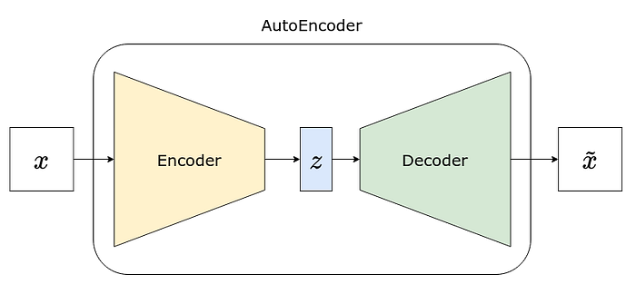
Easy, right? We’re just putting the two pieces together. If we use the models from the previous sections, it looks like this:

AutoEncoder(
  (enc): Encoder(
    (base_model): Sequential(
      (0): Flatten(start_dim=1, end_dim=-1)
      (1): Linear(in_features=784, out_features=2048, bias=True)
      (2): LeakyReLU(negative_slope=0.01)
      (3): Linear(in_features=2048, out_features=2048, bias=True)
      (4): LeakyReLU(negative_slope=0.01)
    )
    (lin_latent): Linear(in_features=2048, out_features=1, bias=True)
  )
  (dec): Sequential(
    (0): Linear(in_features=1, out_features=2048, bias=True)
    (1): LeakyReLU(negative_slope=0.01)
    (2): Linear(in_features=2048, out_features=2048, bias=True)
    (3): LeakyReLU(negative_slope=0.01)
    (4): Linear(in_features=2048, out_features=784, bias=True)
    (5): Unflatten(dim=1, unflattened_size=(1, 28, 28))
  )
)

Moreover, it’s also easy to see that the decoder is a mirror image of the encoder, as shown in the table below:

“Matching” layers as a mirror image. Image by author.

Now, let’s see how we can perform the…

Model Training (AE)

This is a typical training loop in PyTorch: performing the forward pass, computing the loss, computing the gradients using backward(), updating the parameters, and zeroing the gradients. Business as usual!

Epoch 001 | Loss >> 0.1535
Epoch 002 | Loss >> 0.0220
...
Epoch 009 | Loss >> 0.0117
Epoch 010 | Loss >> 0.0109

In case you need a refresher on how to train a model in PyTorch, please check:

Understanding PyTorch with an example: a step-by-step tutorial

Example of Reconstruction

Now that the model was trained, let’s encode, and decode (that is, reconstruct) image #7 from our dataset:

A reconstructed circle. Image by author.

Not so bad, right? The circle was clearly reconstructed, but it looks like some other, smaller, circle was also faintly reconstructed. Let’s try to understand why this is happening…

Latent Space Distribution (AE)

If we plot a histogram of the corresponding latent spaces (z) of each and every image in our dataset, we’ll get the plot on the left. There are a couple of things to notice:

(1) the huge spike slightly below 1 — it means that MANY images in our dataset were mapped into a tiny interval [0.6, 0.9];

(2) all the points are inside the [-0.50, 1.62] — anything outside this interval is “empty” latent space;

Left: distribution of the latent space; Right: latent space versus radius. Image by author.

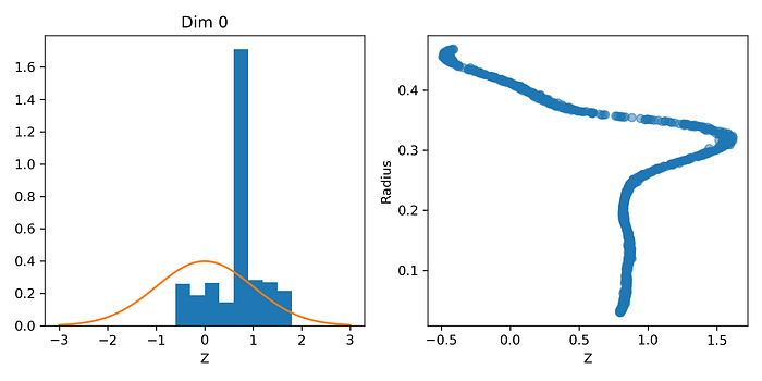
To investigate it further, we can plot the latent spaces against the circle’s radius for each and every image as well, and that’s the plot on the right.

“The radius? Why?”

Since our circles were drawn in the center of the image (apart from a little bit of jiggling), the one feature that best describes a circle is its radius. Our autoencoder’s task was to map circles into a single dimension in the latent space. So, maybe, just maybe, it could have learned to map circles into a latent space that actually represents the radius. That would be awesome, right?

If that were the case, we should see a linear relationship between a circle’s radius and its corresponding one-dimensional latent space. But, clearly, there’s no such relationship anywhere to be seen in the right plot, at least, not for the full range of radiuses (or radii, if you like the Latin plural better!).

What do we find there instead?

(3) circles with a radius less than 0.25 or so were all mapped to the [0.6, 0.9] interval of the latent space (the vertical part of the plot);

(4) for radius between 0.25 and 0.3 or so, there’s a linear relationship between radius and mapped latent space;

(5) for radius above 0.3 or so, there’s roughly a negative linear relationship between radius and mapped latent space.

“What does it mean, in practice?”

Let’s reconstruct some images to illustrate it better!

Reconstruction (AE)

We’re reconstructing five images, corresponding to five points in the latent space (-3.0, -0.5, 0.0, 0.9, 3.0) that may help us understand better what’s happening:

Reconstructed images (AE) for chosen points in the latent space. Image by author.

• [-3.0] and [3.0], are in both ends of “empty” latent space, “where no circle has gone before”, and yet, the autoencoder is still generating circles, although they do seem to have some noise as well;
• [-0.5] and [0.0], sitting at the edge of the mapped latent space, and corresponding to a radius of approximately 0.4, respectively; they are the “success” cases of reconstructed circles, even though they seem to contain a faint, smaller, inner circle too;
• [0.9], corresponding to the “congested” region of the latent space, it looks like a “mixture” of small circles of different radiuses.

“To boldly go where no circle has gone before!”

Captain Picard

We can certainly do better than that, but we need to use better models, namely, variational autoencoders, which is going to be the topic of the second article of this series.

BONUS: AutoEncoders as Anomaly Detectors

This section was inspired by one of the most interesting articles I’ve ever read — “Passing a Chicken through an MNIST Model”, by Emilien Dupont. It illustrates, in great detail, the role autoencoders can play as anomaly detectors.

I will be just scratching the surface of the topic here, so you can get the gist of it. But, instead of a chicken, I decided to use a duck, just because I like ducks better. So, let’s start with a duck, better yet, an MNISTified duck!

A Duck, both high-res, and MNISTified! Adapted from this image from Wikimedia Commons.

“What the duck is that?!”

Clearly, a duck is NOT a circle. Nonetheless, if we feed a 28x28 pixels image of a duck to our encoder, it WILL output the corresponding latent space, no matter what.

“What’s the point of mapping a duck to the latent space of circles?”

The latent space itself is not so interesting, but the reconstructed duck is! If we feed a latent space to our decoder, it WILL output a reconstructed image, no matter what. Let’s see what happens…

Reconstructing a duck — or trying to! Image by author.

Well, the reconstructed image looks much more like a circle than a duck! That shouldn’t be a surprise, after all, we trained our autoencoder on images of circles.

“I don't get it; how is this ‘interesting’?”

The fact that the reconstructed image does not look like the original image at all is quite a strong indication that the original image (a duck) does not belong to the same distribution of data (circles) used to train the autoencoder.

That’s the interesting part — we can use the reconstruction loss (that is, the difference between original and reconstructed images) to classify images as anomalies.

Once you know an image does not belong with the others in the original dataset used for training a model, there’s little or no reason to make predictions using that image as input anymore.

Let’s say we pass our duck through an MNIST model trained to classify digits (that’s what Emilien did in his article). The classifier may predict our duck is a “5” or an “8”, but these predictions are obviously nonsense. The classifier cannot do any better because it is unable to output “I don’t know” as a prediction. But, if we use an autoencoder to detect anomalous inputs — prior to submitting them to another model — we can easily achieve that.

Final Thoughts

Thank you for sticking until the end of this long article :-) But, even though it is a long article, it is only an introduction, and it only covers the fundamental tools and techniques you need to familiar with to start experimenting with autoencoders.

In the second post of this series, we'll learn about variational autoencoders (VAEs), the reparametrization trick, the Kullback-Leibler divergence/loss, and convolutional variational autoencoders (CVAEs).

In the meantime, if you want to learn more about autoencoders and generative models in general, I recommend David Foster’s Generative Deep Learning, from O’Reilly.

And, if you want to learn more about PyTorch, Computer Vision, and NLP, give my own series of books, Deep Learning with PyTorch Step-by-Step, a try :-)

If you have any thoughts, comments, or questions, please leave a comment below or reach out through my bio.link page.

If you like my articles, please consider directly supporting my work by signing up for a Medium membership using my referral page. For every new user, I get a small commission from Medium :-)